Construction Timelapse

In this project a stunning timelapse video was created from an image stock of over 3,000 photos of a construction site, tracking the progress of a new residential building from breaking ground to completion, a process lasting more than three years. Those images were taken without a tripod, so the variability in camera positions and angles was of course high. To correct for this, Computer Vision techniques were used to predict key points in the images, that could then be used to straighten them and produce the final, steady timelapse.

Naturally, this approach required some manual labelling of keypoints in the images, but fortunately I was able to bootstrap these labels to unlabelled images via Computer Vision (or CV, a branch of Machine Learning) by labelling just 10% of the image stock - the rest were labelled by the grace of the predictions from Deep Learning models that I trained.

With those points predicted, the images could be straightened up and stitched together to create a timelapse video of the building as it was being constructed. You can see this (low-resolution) video below. This post will document the technical details of how I went about this, from the initial data labelling to the final video output.

In the end, I made use of fairly traditional CV techniques (convolutions, U-Nets¹, etc.) to arrive at the final product. There are several more² recent³ papers⁴ that I enjoyed reading and would have liked to apply, but that would have been overkill. The two main innovations in this project that helped improve results were:

1. co-learning of multiple keypoints in the same model,
2. making use of 2D Gaussian distributions in the output tensor.

I’ll explain these in more detail below. Without further ado, here is the video:

Music credit: “Our House” by Crosby, Stills, Nash & Young.

Methodology

Code

The convolutional U-Net architecture has now been around for nearly a decade, and is commonly used in tasks where pixel-wise predictions are needed. This is true in our case, since our task is to predict whether each pixel is a keypoint or not - binary classification. I used PyTorch to run the training of the model - a popular Deep Learning package in Python.

I decided to label 12 key points which were mostly points that in theory were visible in every image - even after completion of the building - though some were often occluded. (Two exceptions were two points on the closest crane, which appeared at some point around February 2022 - these were however not used in the end.) Luckily, a reliable group of four keypoints were always in the bottom-left of the images, whilst another four were in the bottom-right. Two models, one for each group, were trained separately. As multiple points were co-learned in the same model, this introduced an extra dimension in the output batch.

Looking for a single point pixel within an image is like trying to find a needle in a haystack, and will surely lead to unstable training. To combat this, I used Gaussian distributions in the output images, centred over the keypoint in question, which made the positive region (much) wider than it would otherwise be with a simple Dirac delta. This method was successful and enabled good progress during model training.

After the trained models were ready, all images were passed through both models to predict keypoints, which allowed the images to be corrected via a translation and rotation using the most confidently predicted keypoints from each group. Images were filtered to choose one frame per day and were further cropped to remove the black borders that were introduced by the affine transformations. Finally, they were stitched together to create the final video that you can enjoy above.

You can see from the next visualization below how much these Machine Learning models have improved the end result - the video shows before (right) and after (left) applying the CV corrections, side-by-side. In the right-hand side showing the uncorrected version, the target building moves around a significant amount:

Data Labelling

In order to have any chance of a usable a model, I had to create a bespoke dataset of labelled images. This was done with the help of the Label Studio tool, which allowed me to quickly label the images with the keypoints that I had chosen. It is easy to set up and use, and runs as a local app in the browser.

The original images had dimension 4032 x 3024, but they were labelled in the lower resolution of 1024 x 768. A total of four months’ worth of images were each labelled with 12 keypoints (Sep & Dec 2021, Mar & Jun 2022), a total of 331 images. This is a mere ~10% fraction of the 3.2k images that were taken throughout the project! Of these, 12% were reserved for the validation dataset.

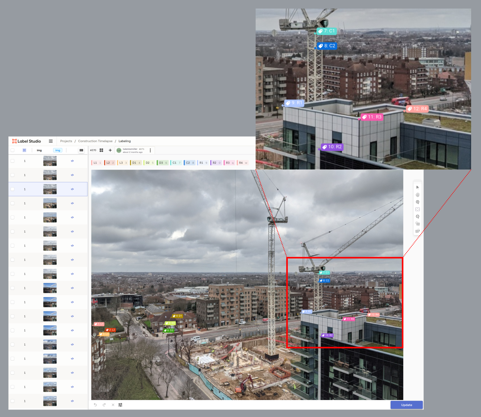
Below is an example of the image-labelling process, captured from Label Studio running in the browser:

The keypoints were:

• C1, C2: points on the smaller crane
• D1, D2, D3: points on the dental surgery opposite
• L1, L2, L3: points on the left-hand building
• R1, R2, R3, R4: points on the right-hand building

Note that L1 and L3 were quite often out of view and therefore were not used. C1 and C2 were not used as they were available in less than half of the labelled images.

Ultimately, only two keypoints were needed in order to adjust the image correctly, but the co-learning of several keypoints together proved invaluable in the training process (more on that later). The two groups were:

• “DL group”: (D1, D2, D3, L1),
• “R group”: (R1, R2, R3, R4).

Inputs & Outputs

The labelled images were cropped into 512 x 512 segments of the low-resolution original, then the upper quadrants were discarded, as all of the action takes place in the lower half of the image. The images were then colour-normalized (using standard ImageNet parameters) prior to entering the models. I chose to avoid image augmentation in the final iteration, as the horizontal flipping seemed to confuse earlier versions of the models.

The image labels were transformed versions of the original 512 x 512 crops - the location of the labelled keypoint was used to construct a 2D Gaussian distribution centred on the keypoint. The standard deviation of the Gaussian was fairly tight, with a value of just two pixels. Each keypoint in the group had its own greyscale “output image” (which you can imagine to be mostly black with a small white circle where the keypoint is). The values were normalized to be in the interval [0, 1].

Those are stacked together to form 4D output tensors:

(batch size, keypoints, height, width) = (12, 4, 512, 512)

which were used to train the model with a binary cross-entropy loss (averaged across the dimensions).

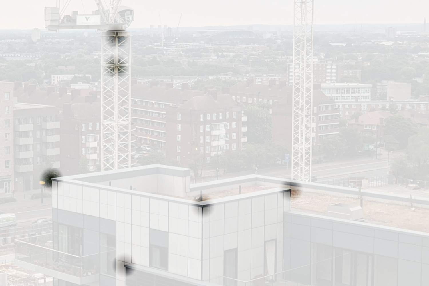
For visualisation purposes, in the image below you can see part of an example frame where the opacity is proportioned according to the intensity of the pixels’ labels (via the Gaussian distribution), making the background mostly translucent. Note that I have used the wider sigma value of 25 pixels so that the keypoints can be seen more clearly. (Click to zoom.)

The validation set was formed by md5-hashing the date of the image, then choosing those whose hash value ended with the hexidecimal digit ‘2’ or ‘3’ (about 12.5% in expectation). In this way, all images from the same day had to be strictly within either the training or validation set, thereby preventing leakage.

Architecture & Training

I chose the U-Net architecture for the model, as it is capable of producing per-pixel predictions. The input batches pass through four encoder layers before hitting the bottleneck, and then exit via four decoder layers. BatchNorm was used throughout the architecture, along with ReLU activations. The final layer was a sigmoid activation, producing probability outputs between 0 and 1, where values near 1 are indicative of a keypoint.

As mentioned earlier, there were two models trained - one for the “DL group” and one for the “R group”. The models were trained separately on GPU spot instances of type p3.2xlarge on AWS. As the GPU memory was limited, it could only manage a maximal batch size of 12. There was a dramatic acceleration in training time when the models were trained on the GPU, as you might expect. By CV standards, this dataset is not huge, but nonetheless per-epoch time was approx. 30 minutes on my (fairly powerful) laptop, compared to between 15-25 seconds on the cloud GPU machine. Below is an excerpt from the training logs of the DL group model:

---------EPOCH 0---------
	(2024-11-15 17:42:46):    VAL: batch 001
                                                       loss: 49.730617
                                                       n-way loss: [50.7885 49.9106 49.797  48.4264]
                                                       max_metric: [0.5161 0.5056 0.5045 0.4919]

	(2024-11-15 17:43:11):    VAL: batch 025
                                                       loss: 1.275463
                                                       n-way loss: [1.3868 1.421  1.4029 0.8912]
                                                       max_metric: [0.1287 0.1253 0.1443 0.0982]
---------EPOCH 1---------
	(2024-11-15 17:43:27):    VAL: batch 025
                                                       loss: 0.250573
                                                       n-way loss: [0.2452 0.248  0.3005 0.2086]
                                                       max_metric: [0.0115 0.0116 0.0149 0.0083]
---------EPOCH 2---------
	(2024-11-15 17:43:44):    VAL: batch 025
                                                       loss: 0.157465
                                                       n-way loss: [0.1535 0.1551 0.1866 0.1347]
                                                       max_metric: [0.0045 0.0045 0.0063 0.0035]
---------EPOCH 3---------
	(2024-11-15 17:44:01):    VAL: batch 025
                                                       loss: 0.117230
                                                       n-way loss: [0.1144 0.1151 0.1386 0.1008]
                                                       max_metric: [0.0032 0.0032 0.0045 0.0025]
---------EPOCH 4---------
	(2024-11-15 17:44:18):    VAL: batch 025
                                                       loss: 0.091978
                                                       n-way loss: [0.0898 0.0905 0.1086 0.0791]
                                                       max_metric: [0.0026 0.0026 0.0036 0.0021]
...
---------EPOCH 147---------
	(2024-11-15 18:23:49):    VAL: batch 025
                                                       loss: 0.001135
                                                       n-way loss: [0.0012 0.0011 0.0012 0.001 ]
                                                       max_metric: [0.7684 0.814  0.8005 0.698 ]
---------EPOCH 148---------
	(2024-11-15 18:24:05):    VAL: batch 025
                                                       loss: 0.001160
                                                       n-way loss: [0.0012 0.0012 0.0012 0.0011]
                                                       max_metric: [0.8017 0.8102 0.8103 0.7288]
---------EPOCH 149---------
	(2024-11-15 18:24:22):    VAL: batch 025
                                                       loss: 0.001130
                                                       n-way loss: [0.0012 0.0011 0.0012 0.001 ]
                                                       max_metric: [0.7752 0.8183 0.8123 0.7028]

You can see in the log that as well as the global loss continuing to generally decrease, the 4-way loss (one for each keypoint) also remained fairly balanced with no one keypoint dominating the others. This gave me the confidence to use all keypoints as prediction candidates.

Validation loss continued to decrease through 150 epochs, but I capped it there as the gains were becoming minimal (and GPU time is somewhat expensive!).

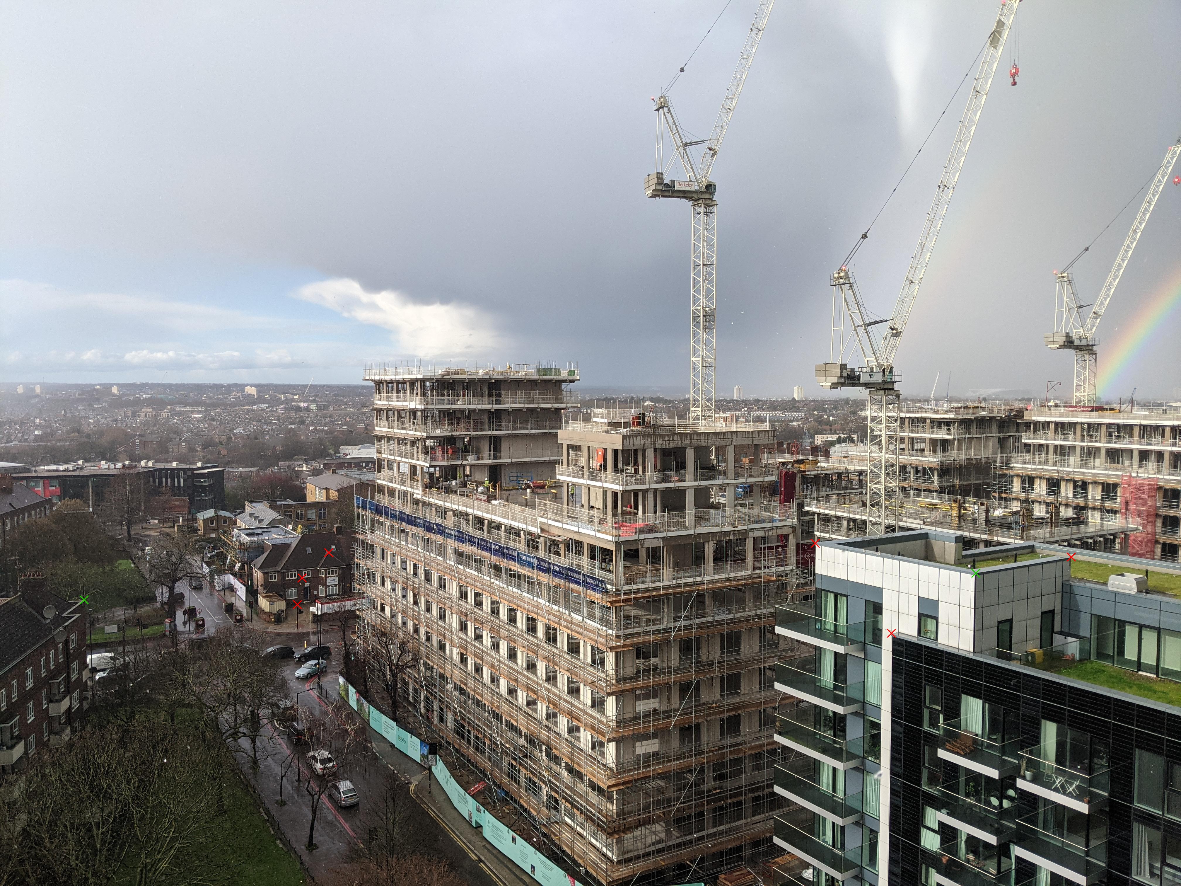
Below is an example of the models’ predictions on an unseen image (click to zoom):

All crosses represent predicted keypoints - the green ones were the most confident predictions from each group and were used to correct the frame.

Post-Hoc Adjustments

Having obtained the predicted locations of the keypoints of all images, we need to put them to use. One frame per day was selected, and then the keypoint with the highest confidence from each model was used to parametrize the translation and rotation operations. It was important to take one from each group (one on the left, one on the right) since small prediction errors can be exaggerated if keypoints are too close.

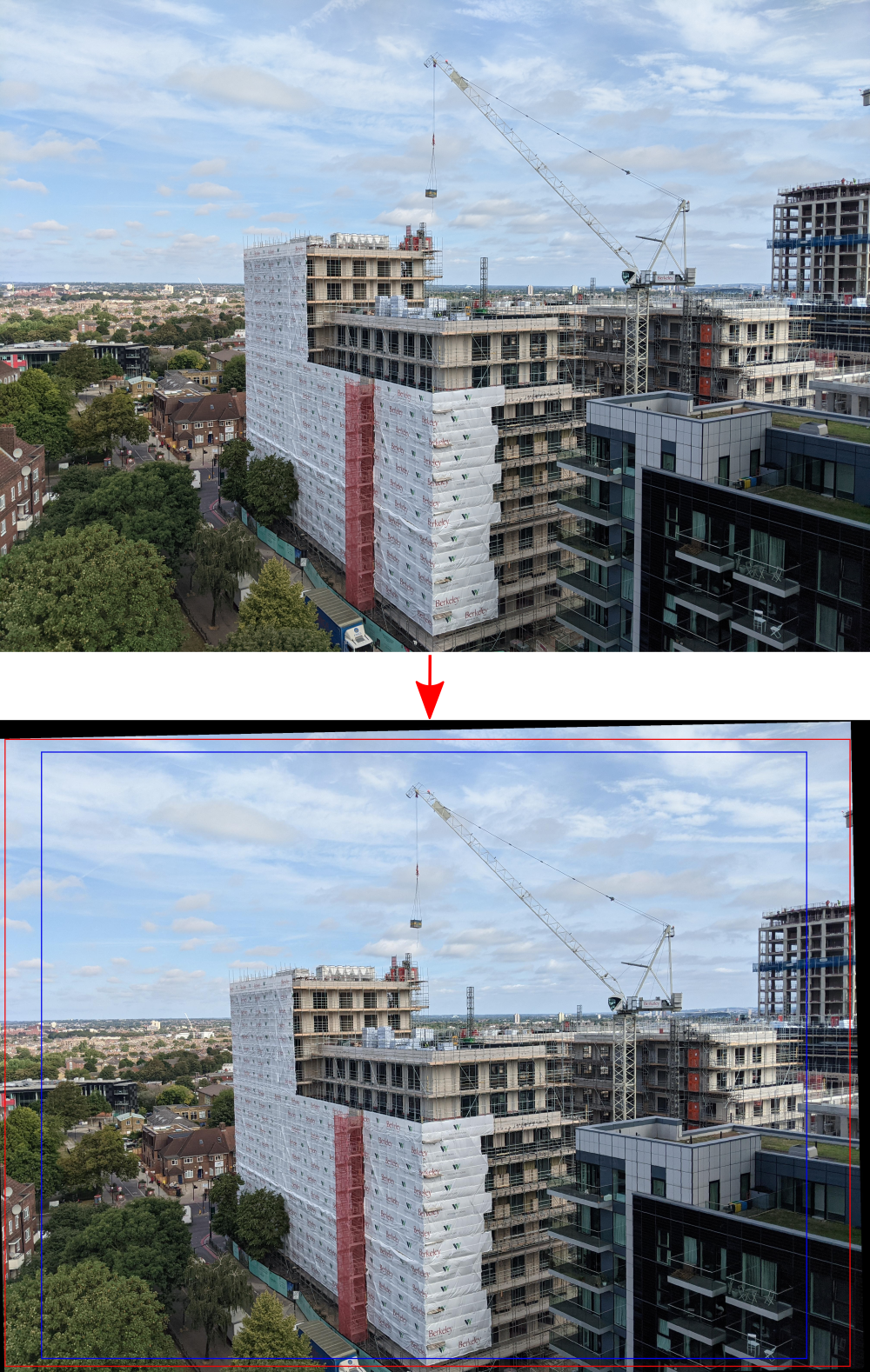
To be explicit, the image was translated to first fix the right-hand keypoint to its expected location, then the image was rotated about this point to fix the left-hand keypoint. As you can see from the example below, this typically introduces - to a varying degree - black borders at the edges. The frames for the final video were cropped such that it would remove these borders from all the chosen images.

Here is an example showing the adjustment operations compared to the original image:

You can see that the rotation has created a black border along the top and right edges, which would be removed by the red cropping box in this example. Other instances shrink the cropping region even further and the blue box shows the maximal cropping extent for all selected images, in order to avoid black regions appearing anywhere.

Finally, the images were stitched together with ffmpeg at a frame rate of 10 fps and watermarked to produce the final video that you see above.

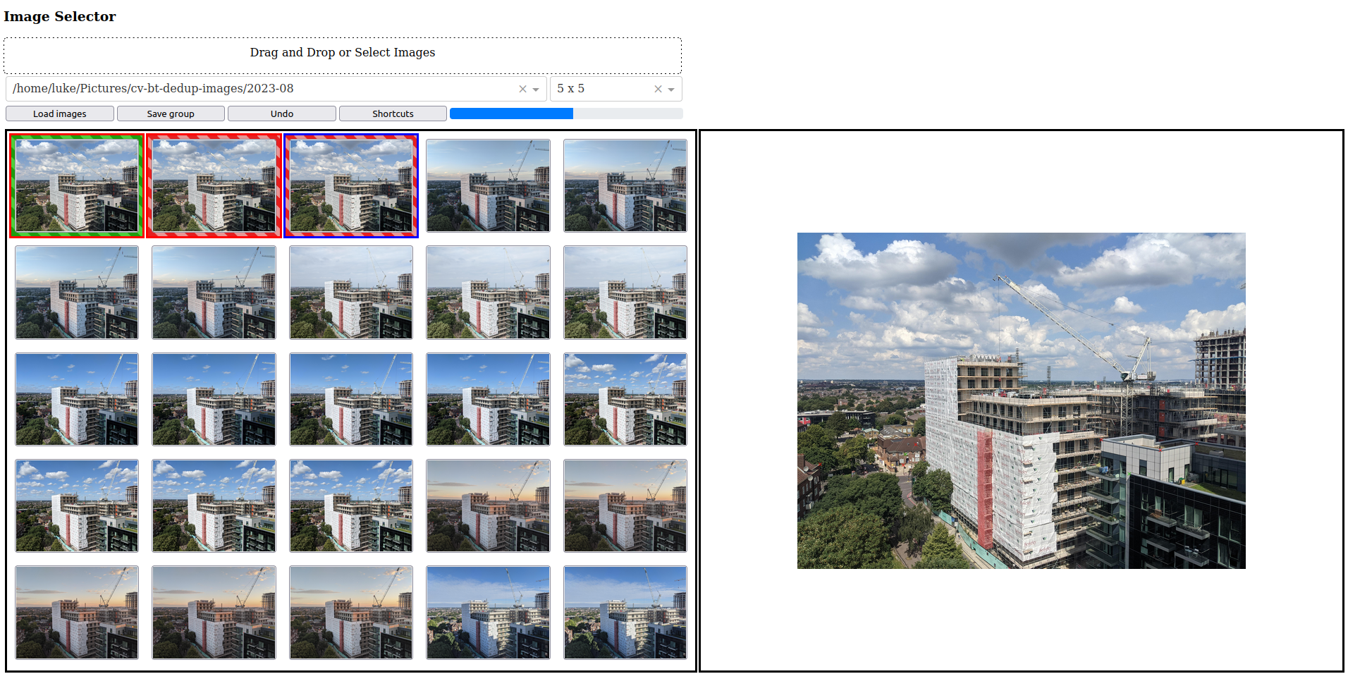
One final note in this section is that I made use of my earlier “Image Selector” project to choose the best frame per day. You can see an example of how this worked in the image below, or you can read more about that project here.

Outtakes

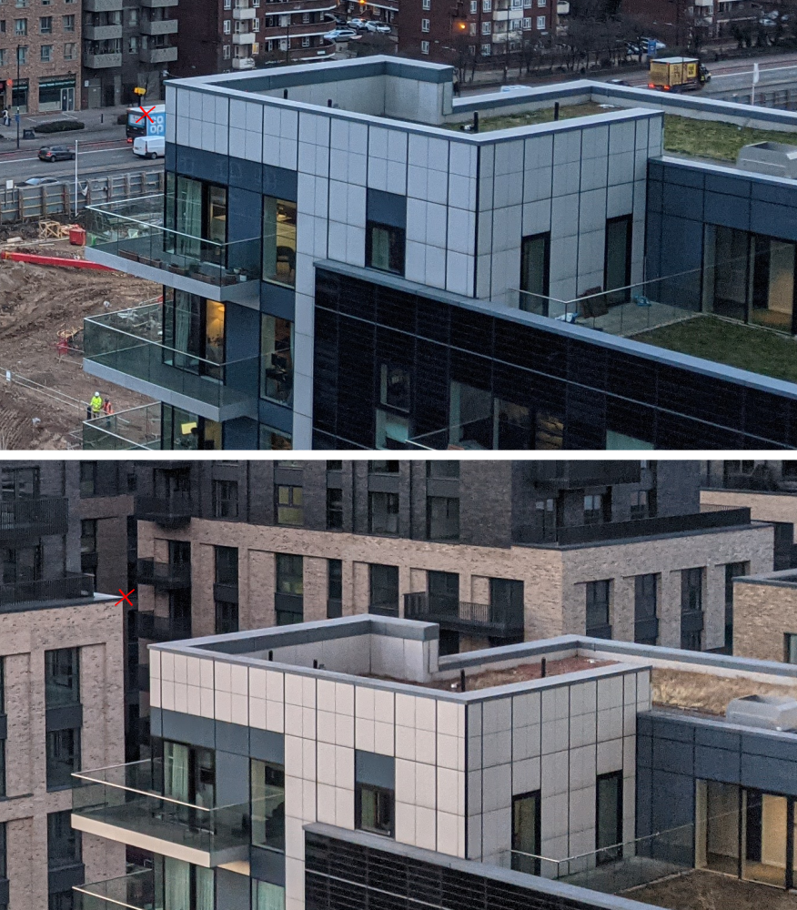
The first round of training consisted of using singular models for each keypoint separately, but this led to regular (and sometimes amusing) mistakes when predicting on out-of-sample images. The examples below show:

1. the R3 model confusing a passing truck with the correct corner of the building (uncanny similarity!) (top) and
2. the R1 model predicting a nearby corner of the target building once built (bottom).

I believe these types of mistakes were unlikely in the 4-way co-learnt models as the network was able to learn some sense of relative distance to other keypoints. Also, I removed horizontal flip augmentation to prevent reflective mistakes as in 2.

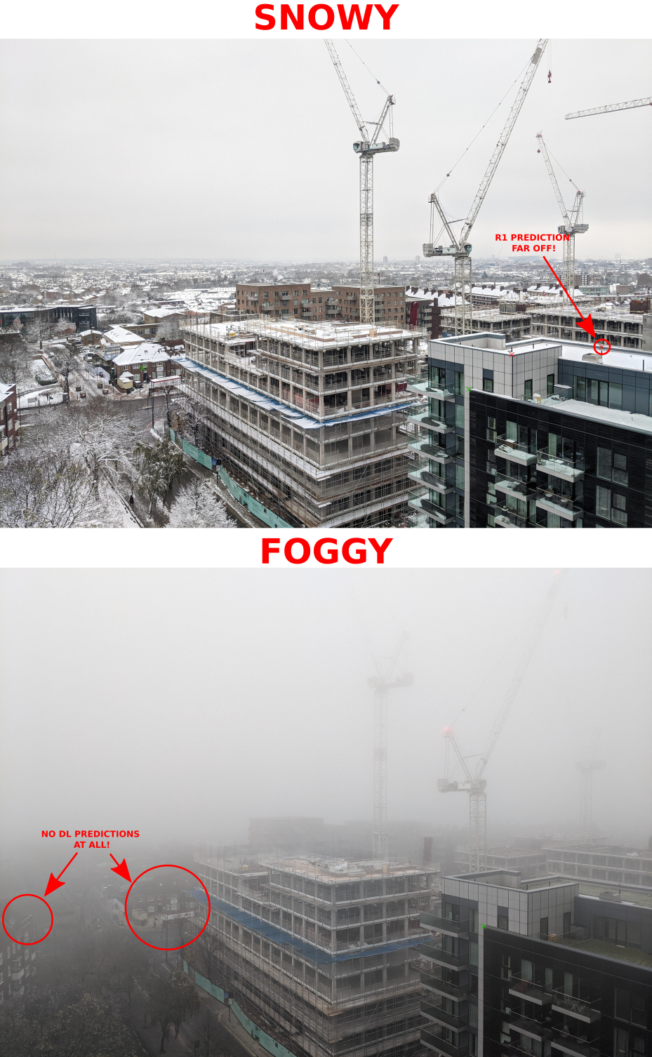
The next category of mistakes were caused by adverse weather conditions, such as snow and fog as seen in the example below. These didn’t occur too often and so were easy to correct with manual labels.

Lessons Learned

In this project, some of my key takeaways were:

• The use of co-learning of multiple keypoints in the same model was a very helpful addition - it allowed to U-Net to learn relative distances between keypoints, preventing easy mistakes that the initial single-keypoint models were liable to.
• Experimentation and the iteration of ideas does take time, but ultimately delivers a good solution.
• Next time, use a tripod 😅

If you like this project, please hit the ⭐ button on the GitHub page!

This project was a great learning experience for me, and I hope that you find it interesting too. If you have any questions, please don’t hesitate to get in touch via the contact page.

• ComputerVision
• Video
• MachineLearning
• Python
• PyTorch